 |
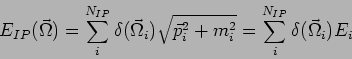
(1) |
The charged tracks change their initial direction due to the bending in the strong magnetic field that leads to jet energy flux distortion at the calorimeter inner surface.
The energy flux at the calorimeter surface
![]() can be written as:
can be written as:
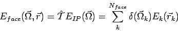 |
(2) |
The energy deposition distribution in the calorimeter volume
![]() can be written as:
can be written as:
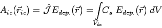
| (3) |
The operator ![]() can be formally represented as a sum of
operators of separated particle types (ID) with different behaviour in
the calorimeter.
can be formally represented as a sum of
operators of separated particle types (ID) with different behaviour in
the calorimeter.
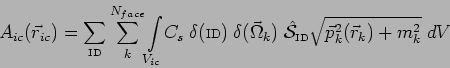
| (4) |
 |
(5) |
After substitutions we have the set of equations for
![]() that are measurable amplitudes at the center
that are measurable amplitudes at the center
![]() of electronic cell volume
of electronic cell volume ![]() :
:
 |
(6) |
The backward problem for this system of equations is the particle-flow
reconstruction problem.
It was solved in some way for many different HEP detectors.
Analogs of such a kind of problem (successfully solved!) are the adjoint problem for the design of nuclear power reactors and the image reconstruction in the modern gamma-chamber in nuclear medicine.
Taking into account the definition of operator ![]() one can
recognize well known calorimeter energy-flow formula in this
equations, that is a sum of energy over all calorimeter cells:
one can
recognize well known calorimeter energy-flow formula in this
equations, that is a sum of energy over all calorimeter cells:
![]() .
.
In reality any calorimeter cell can carry the signals from many initial particles!
A few more remarks on this problem:
These formulae are the strict mathematical definition of the bootstrap method for the fast simulation programs.
The equations can be rewritten as a sum of charged and neutral
particles separately with the parameterization of shower operators
![]() to make an analytical investigation of its
properties.
to make an analytical investigation of its
properties.
If one reduces the cell volume up to zero the overlapping still would take place for the shower volume.
At this stage of the investigation of the equations they are not solved directly, but as it was said early, they were solved indirectly in many HEP experiments.
TESLA calorimeter reconstruction program SNARK is one of such a solution.
![\includegraphics[width=0.8\textwidth]{Vector.eps}](img46.png) |
The idea of solution is based on the shape of the shower operator
![]() straightforward. If one have the
``exactly'' (with very good accuracy) measured particle energy and its
direction - so, one can take this knowledge and looks for the
calorimeter hits along the predicted particle direction and separates
this part of event from the others, that is clear but for
the fine calorimeter cell structure only.
straightforward. If one have the
``exactly'' (with very good accuracy) measured particle energy and its
direction - so, one can take this knowledge and looks for the
calorimeter hits along the predicted particle direction and separates
this part of event from the others, that is clear but for
the fine calorimeter cell structure only.
![\includegraphics[width=0.8\textwidth]{shell.eps}](img48.png) |
The algorithm starts from the finding the charged track core. The track core is the collection of the calorimeter hits which are at the distances less then one cell size from the extrapolation of the TPC measured track (helix curve) into the calorimeter volume.
Such a procedure works well for the muon track with energy more then
2 GeV (at 3 Tesla), for the lower energy a helix can be replaced by
more sophisticated curve with taking into account the energy
losses. It also works well for the primary ionization part of the
hadron track (that is about 20 % of whole deposited energy in the
hadron shower). It also works for the electromagnetic shower but due
to the fact that the electromagnetic shower is rather short
(![]() 20 cm) and transversally compact in W-Si structure of TESLA ECAL.
20 cm) and transversally compact in W-Si structure of TESLA ECAL.
The track core collects almost all hits for muon track, the main part of hadron track primary ionization and rather big part of the electromagnetic shower. The longitudinal distribution and average density of hits can be tested for different particle hypothesis even at the level of track core collection.
The next step of the procedure is based on the previous knowledge and estimations; it is the hit collection around the track core at the distances of two cell sizes - called first shell (see picture).
The particle identification is repeated for the new cluster that includes as a track core as a first shell and ... so on.
The iterative procedure is finished when the collected energy become to be ``equal'' to the input particle momentum. For the muon hypothesis procedure is stopped just after the first step. The word ``equal'' means equal inside the calorimeter energy resolution, more exactly it is particle momentum plus/minus tuning parameters that depend on input energy, calorimeter sampling and particle hypothesis. We will not describe here in details all cases that program trying to resolve during the iterative procedure - its number is about 35 for now. There are different particle hypothesis and their combinations with taking into account the showers overlapping (one can see the text of program).
At the end of loop around charged tracks all hits belong to them are collected in clusters, labeled and they will not use more at the next step of the reconstruction.
The program starts the procedure to collect and separate the neutral part of event after the collecting all clusters for charged particles.
This algorithm applied the hit histograming technique in ![]() space to find at first the super-clusters then clusters inside the
super-clusters.
space to find at first the super-clusters then clusters inside the
super-clusters.
Then it collects additional hits around the core of found clusters and it try to create the for every neutral particle as hadron as electromagnetic one.
The super-clusters in ![]() coordinate space are constructed
by combining all calorimeter hits which are within a certain distance
coordinate space are constructed
by combining all calorimeter hits which are within a certain distance
![]() in
in ![]() space. If two super clusters overlap, the
energy inside the overlapped region is assigned to both
super-clusters weighted by the total energy of the respective
super-cluster. The properties of the super-cluster are calculated:
energy, center position and angular radius.
space. If two super clusters overlap, the
energy inside the overlapped region is assigned to both
super-clusters weighted by the total energy of the respective
super-cluster. The properties of the super-cluster are calculated:
energy, center position and angular radius.
Clusters inside the super-cluster are reconstructed by combining
hits assigned to the super-cluster which are within a certain distance
![]() in
in ![]() space. For the overlapping
clusters the same method as above is applied. Then the cluster
properties are calculated: energy, number of hits, hit density, center
position, principal cluster axes, parameters of electromagnetic shower
hypothesis.
space. For the overlapping
clusters the same method as above is applied. Then the cluster
properties are calculated: energy, number of hits, hit density, center
position, principal cluster axes, parameters of electromagnetic shower
hypothesis.
Each cluster is assigned to a particle type based on its predicted and calculated shape parameters for gamma or hadron hypothesis. The remaining hits are joined to the closest cluster. The clusters whose main axes are overlapping within a certain window are merged into one cluster. Finally all cluster properties are recalculated.
This procedure is done for both ECAL and HCAL separately. ECAL and HCAL clusters are joined if they match a certain criteria.
Assuming that the cluster profile in transverse direction can be
described by an exponential law, the cluster shape in a logarithmic
![]() space is simple a cone. If two clusters overlap, the
energy of cells in the overlap region is assigned to both clusters,
weighted by the linear distance to the respective cluster axis. In
the current version of the software up to six clusters are allowed to
overlap, at most three in one point.
space is simple a cone. If two clusters overlap, the
energy of cells in the overlap region is assigned to both clusters,
weighted by the linear distance to the respective cluster axis. In
the current version of the software up to six clusters are allowed to
overlap, at most three in one point.